In probability theory and statistics, Bayes’ theorem, named after Thomas Bayes, describes the probability of an event, based on prior knowledge of conditions that might be related to the event. For example, if the risk of developing health problems is known to increase with age, Bayes’ theorem allows the risk to an individual of a known age to be assessed more accurately (by conditioning it on their age) than simply assuming that the individual is typical of the population as a whole.
Statement of theorem
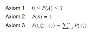
Bayes’ theorem is stated mathematically as the following equation:
![\[ P(A|B)=\frac{P(B|A)P(A)}{P(B)} \]](https://emanueleseminara.it/wp-content/ql-cache/quicklatex.com-f1a041584951e962ba9a4f3bc776da6e_l3.png "Rendered by QuickLaTeX.com")
where A and B are events and 
 is a conditional probability: the probability of event
  occurring given that
  is true. It is also called the posterior probability of given .
 is also a conditional probability: the probability of event occurring given that is true. It can also be interpreted as the likelihood of given a fixed because
  .
. and
and  are the probabilities of observing and respectively without any given conditions; they are known as the marginal probability or prior probability.
- and must be different events.
There are several paradigms within statistical inference such as:
- early Bayesian inference;
- Fisherian inference;
- Neyman-Pearson inference;
- Neo-Bayesian inference;
- Likelihood inference.
Early Bayesian inference
Bayesian inference refers to the English clergyman Thomas Bayes (1702-1761), who was the first who
attempted to use probability calculus as a tool for inductive reasoning, and gave his name to what later became known as Bayes law. However, the one who essentially laid the basis for Bayesian inference was the French mathematician Pierre Simon Laplace (1749-1827). This amounts to having a non-informative prior distribution on the unknown quantity of interest, and with observed data, update the prior by Bayes law, giving a posterior distribution where the expectation (or mode) could be taken as an estimate of the unknown quantity. This way of reasoning was frequently called inverse probability and was picked up by Gauss (1777-1855).
Fisherian inference
The major paradigm change came with Ronald A. Fisher (1890-1962), probably the most influential statistician of all times, who laid the basis for a quite different type of objective reasoning. About 1922 he had concluded that inverse probability was not a suitable scientific paradigm. In his words a few years later “the theory of inverse probability is founded upon an error, and must be wholly rejected”.
Instead, he advocated the use of the method of maximum likelihood and demonstrated its usefulness as well as its theoretical properties. One of his supportive arguments was that inverse probability gave different results depending on the choice of parameterization, while the method of maximum likelihood did not, e.g. when estimating unknown odds instead of the corresponding probability. Fisher clarified the notion of a parameter, and the difference between the true parameter and its estimate, which had often been confusing for earlier writers. He also separated the concepts of probability and likelihood and introduced several new and important concepts, most notably information, sufficiency, consistency, and efficiency.
Neyman-Pearson inference
In the late 1920s, the duo Jerzy Neyman (1890-1981) and Egon Pearson (1895-1980) arrived on the scene.
They are largely responsible for the concepts related to confidence intervals and hypothesis testing. Their ideas had a clear frequentist interpretation, with significance level and confidence level as risk and covering probabilities attached to the method used in repeated application. While Fisher tested a hypothesis with no alternative in mind, Neyman and Pearson pursued the idea of test performance against specific alternatives and the uniform optimality of tests. Moreover, Neyman imagined a wider role for tests as a basis for decisions: “Tests are not rules for inductive inference, but rules of behavior”. Fisher strongly opposed these ideas as the basis for scientific inference, and the fight between Fisher and Neyman went on for decades.
Neo-Bayesian inference
In the period 1920-1960, the Bayes position was dormant, except for a few writers. Important for the reawakening of Bayesian ideas was the new axiomatic foundation for probability and utility, established by von Neumann and Morgenstern (1944). This was based on axioms of coherent behavior. When Savage and his followers looked at the implications of coherency for statistics, they demonstrated that a lot of common statistical procedures, although fair within the given paradigm, they were not coherent. On the other hand, they demonstrated that a Bayesian paradigm could be based on coherency axioms, which implied the existence of (subjective) probabilities following the common rules of probability calculus. Of interest here is also the contributions of Howard Raiffa (1924-) and Robert Schlaifer (1914-1994) who looked at statistics in the context of business decisions.
Likelihood inference
This paradigm is one of the five with the shortest history and is formulated by statisticians George Barnard (1915-2002), Alan Birnbaum (1823-1976), and Anthony Edwards (1935-). They also found the classical paradigms unsatisfactory, but for different reasons than the Bayesians. Their concern was the role of statistical evidence in scientific inference, and they found the decision-oriented classical paradigm sometimes worked against a reasonable scientific process. The Likelihoodists saw it as a necessity to have a paradigm that provides a measure of evidence, regardless of prior probabilities and regardless of available actions and their consequences. Moreover, this measure should reflect the collection of evidence as a cumulative process. They found the classical paradigms (Neyman-Pearson or Fisher) with its significance levels and P-values not able to provide this, and they argued that evidence of observations for a given hypothesis has to be judged against an alternative (and thus Fishers claim that P-values fairly represent a measure of evidence is invalid). They suggested instead to base the scientific reporting on the likelihood function itself and use likelihood ratios as measures of evidence. This gives a kind of plausibility guarantee, but no direct probability guarantees as with the other paradigms, except that probability considerations, can be performed when planning the investigation and its size.


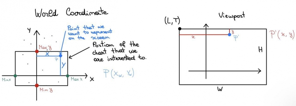
![\[ \begin{cases} x= f_x(x_w)\\ y=f_y(y_w) \\ \end{cases} \]](https://emanueleseminara.it/wp-content/ql-cache/quicklatex.com-2d81facabf1bd6790d766ddd9de4f409_l3.png "Rendered by QuickLaTeX.com")
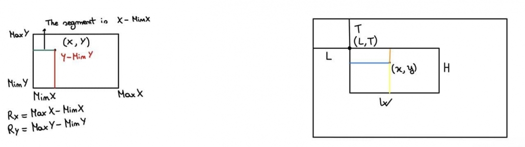
![\[ x=L+\frac{x-x_{min}}{R_x}\cdot w \]](https://emanueleseminara.it/wp-content/ql-cache/quicklatex.com-7244a381fedf08d95591af1b229f78a3_l3.png "Rendered by QuickLaTeX.com")
![\[ y=T+H-\frac{y-y_{min}}{R_y}\cdot h \]](https://emanueleseminara.it/wp-content/ql-cache/quicklatex.com-7460564b211a3124bdcf7845e716bb60_l3.png "Rendered by QuickLaTeX.com")
![\[\bar{x}=\sum \frac{x_i}{n}\]](https://emanueleseminara.it/wp-content/ql-cache/quicklatex.com-950b7b3efc2307fe4e3744ee34bd1bda_l3.png "Rendered by QuickLaTeX.com")
![\[D(x, y)=\sqrt{\sum_{i=1}^n (x_i-y_i)^2}\]](https://emanueleseminara.it/wp-content/ql-cache/quicklatex.com-67b4d5709eb12fed6e00f6e67f6c196e_l3.png "Rendered by QuickLaTeX.com")
:max_bytes(150000):strip_icc():format(webp)/bar-chart-build-of-multi-colored-rods-114996128-5a787c8743a1030037e79879.jpg)
:max_bytes(150000):strip_icc():format(webp)/pie-chart-102416304-59e21f97685fbe001136aa3e.jpg)
:max_bytes(150000):strip_icc():format(webp)/Travel_time_histogram_total_1_Stata-5a788217d8fdd500372f00fd.png)
:max_bytes(150000):strip_icc():format(webp)/Scatterplot_and_LOESS_of_Relative_WikiWork_Score_and_Number_of_Assessed_Articles-5a788083ff1b780037f1ca63.png)
:max_bytes(150000):strip_icc():format(webp)/Edgcott_Population_Time_Series_Graph-5a78812b642dca0037c46c59.jpg)