This example shows how to generate random numbers using the uniform distribution inversion method. This is useful for distributions when it is possible to compute the inverse cumulative distribution function, but there is no support for sampling from the distribution directly.
Step 1. Generate random numbers from the standard uniform distribution.
Use rand to generate 1000 random numbers from the uniform distribution on the interval (0,1).
rng('default')  % For reproducibility
u = rand(1000,1);
The inversion method relies on the principle that continuous cumulative distribution functions (CDFs) range uniformly over the open interval (0,1). If u is a uniform random number on (0,1), then x=F−1(u) generates a random number x from any continuous distribution with the specified cdf F.
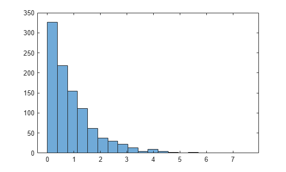
Step 2. Generate random numbers from the Weibull distribution.
Use the inverse cumulative distribution function to generate the random numbers from a Weibull distribution with parameters A = 1 and B = 1 that correspond to the probabilities in u. Plot the results.
x = wblinv(u,1,1);
histogram(x,20);
The histogram shows that the random numbers generated using the Weibull inverse CDF function wblinv have a Weibull distribution.
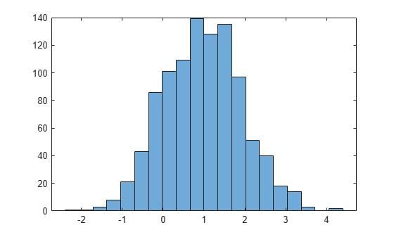
Step 3. Generate random numbers from the standard normal distribution.
The same values in u can generate random numbers from any distribution, for example, the standard normal, by following the same procedure using the inverse CDF of the desired distribution.
x_norm = norminv(u,1,1);
histogram(x_norm,20)
The histogram shows that, by using the standard normal inverse CDF norminv, the random numbers generated from u now have a standard normal distribution.
In probability theory and statistics, Bayes’ theorem, named after Thomas Bayes, describes the probability of an event, based on prior knowledge of conditions that might be related to the event. For example, if the risk of developing health problems is known to increase with age, Bayes’ theorem allows the risk to an individual of a known age to be assessed more accurately (by conditioning it on their age) than simply assuming that the individual is typical of the population as a whole.
Statement of theorem
Bayes’ theorem is stated mathematically as the following equation:
where A and B are events and
is a conditional probability: the probability of event occurring given that is true. It is also called the posterior probability of given .
is also a conditional probability: the probability of event occurring given that is true. It can also be interpreted as the likelihood of given a fixed because .
and are the probabilities of observing and respectively without any given conditions; they are known as the marginal probability or prior probability.
and must be different events.
There are several paradigms within statistical inference such as:
early Bayesian inference;
Fisherian inference;
Neyman-Pearson inference;
Neo-Bayesian inference;
Likelihood inference.
Early Bayesian inference
Bayesian inference refers to the English clergyman Thomas Bayes (1702-1761), who was the first who
attempted to use probability calculus as a tool for inductive reasoning, and gave his name to what later became known as Bayes law. However, the one who essentially laid the basis for Bayesian inference was the French mathematician Pierre Simon Laplace (1749-1827). This amounts to having a non-informative prior distribution on the unknown quantity of interest, and with observed data, update the prior by Bayes law, giving a posterior distribution where the expectation (or mode) could be taken as an estimate of the unknown quantity. This way of reasoning was frequently called inverse probability and was picked up by Gauss (1777-1855).
Fisherian inference
The major paradigm change came with Ronald A. Fisher (1890-1962), probably the most influential statistician of all times, who laid the basis for a quite different type of objective reasoning. About 1922 he had concluded that inverse probability was not a suitable scientific paradigm. In his words a few years later “the theory of inverse probability is founded upon an error, and must be wholly rejected”.
Instead, he advocated the use of the method of maximum likelihood and demonstrated its usefulness as well as its theoretical properties. One of his supportive arguments was that inverse probability gave different results depending on the choice of parameterization, while the method of maximum likelihood did not, e.g. when estimating unknown odds instead of the corresponding probability. Fisher clarified the notion of a parameter, and the difference between the true parameter and its estimate, which had often been confusing for earlier writers. He also separated the concepts of probability and likelihood and introduced several new and important concepts, most notably information, sufficiency, consistency, and efficiency.
Neyman-Pearson inference
In the late 1920s, the duo Jerzy Neyman (1890-1981) and Egon Pearson (1895-1980) arrived on the scene.
They are largely responsible for the concepts related to confidence intervals and hypothesis testing. Their ideas had a clear frequentist interpretation, with significance level and confidence level as risk and covering probabilities attached to the method used in repeated application. While Fisher tested a hypothesis with no alternative in mind, Neyman and Pearson pursued the idea of test performance against specific alternatives and the uniform optimality of tests. Moreover, Neyman imagined a wider role for tests as a basis for decisions: “Tests are not rules for inductive inference, but rules of behavior”. Fisher strongly opposed these ideas as the basis for scientific inference, and the fight between Fisher and Neyman went on for decades.
Neo-Bayesian inference
In the period 1920-1960, the Bayes position was dormant, except for a few writers. Important for the reawakening of Bayesian ideas was the new axiomatic foundation for probability and utility, established by von Neumann and Morgenstern (1944). This was based on axioms of coherent behavior. When Savage and his followers looked at the implications of coherency for statistics, they demonstrated that a lot of common statistical procedures, although fair within the given paradigm, they were not coherent. On the other hand, they demonstrated that a Bayesian paradigm could be based on coherency axioms, which implied the existence of (subjective) probabilities following the common rules of probability calculus. Of interest here is also the contributions of Howard Raiffa (1924-) and Robert Schlaifer (1914-1994) who looked at statistics in the context of business decisions.
Likelihood inference
This paradigm is one of the five with the shortest history and is formulated by statisticians George Barnard (1915-2002), Alan Birnbaum (1823-1976), and Anthony Edwards (1935-). They also found the classical paradigms unsatisfactory, but for different reasons than the Bayesians. Their concern was the role of statistical evidence in scientific inference, and they found the decision-oriented classical paradigm sometimes worked against a reasonable scientific process. The Likelihoodists saw it as a necessity to have a paradigm that provides a measure of evidence, regardless of prior probabilities and regardless of available actions and their consequences. Moreover, this measure should reflect the collection of evidence as a cumulative process. They found the classical paradigms (Neyman-Pearson or Fisher) with its significance levels and P-values not able to provide this, and they argued that evidence of observations for a given hypothesis has to be judged against an alternative (and thus Fishers claim that P-values fairly represent a measure of evidence is invalid). They suggested instead to base the scientific reporting on the likelihood function itself and use likelihood ratios as measures of evidence. This gives a kind of plausibility guarantee, but no direct probability guarantees as with the other paradigms, except that probability considerations, can be performed when planning the investigation and its size.
https://emanueleseminara.it/wp-content/uploads/2021/10/Statistics_researches_Research_7R.png705705zifrohttps://emanueleseminara.it/wp-content/uploads/2021/09/logo.pngzifro2021-10-27 18:52:262021-11-08 13:50:17Research about theory 7_R
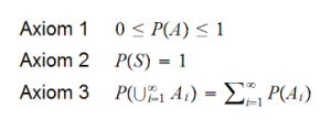
As Kolmogorov said, the probability is an axiom, based on measure theory. The measure is a quantity defined onset, (non-negative, is zero on the empty set, countable additivity).
Given a set X, a power set P(X) (a set of all subsets of all subsets of X), we have a Sigma algebra which is defined as a subset of the power set of x which has some properties.
Probability is a particular case of measure with a particular property, it’s defined between a range (0,1), this range is called the Probability Space. The probability space is represented as triples (Ω, a, p) as in the measure space, where the triples are ( X, Σ, μ).
Ω: is a set of all elements, a: is the sigma-algebra on the set X, p is the probability function.
Starting from empirical objects, I can derive an infinite number of models (theoretical models), defined by the Θ parameter (state of nature) and from these, I can calculate the most probable model, thanks to the role that probability has in statistics.
Introduction
Probability and statistics, the branches of mathematics concerned with the laws governing random events, including the collection, analysis, interpretation, and display of numerical data. Probability has its origin in the study of gambling and insurance in the 17th century, and it is now an indispensable tool of both social and natural sciences. Statistics may be said to have its origin in census counts taken thousands of years ago; as a distinct scientific discipline, however, it was developed in the early 19th century as the study of populations, economies, and moral actions and later in that century as the mathematical tool for analyzing such numbers.
The assumptions as to set up the axioms can be summarised as follows:
Let (Ω, F, P) be a measure space with P(E) being the probability of some event E, and P(Ω) = 1.
Then (Ω, F, P) is a probability space, with sample space Ω, event space F and probability measure P.
First axiom
The probability of an event is a non-negative real number:
where F is the event space. It follows that P(E) is always finite, in contrast with more general measure theory. Theories that assign a negative probability to relax the first axiom.
Second axiom
This is the assumption of unit measure: that the probability that at least one of the elementary events in the entire sample space will occur is 1
P(Ω) = 1
Third axiom
This is the assumption of σ-additivity:
Any countable sequence of disjoint sets (synonymous with mutually exclusive events) E1, E2, . . . . satisfies
Many important laws are derived from Kolmogorov’s three axioms. For example, the Law of Large Numbers can be deduced from the laws by logical reasoning (Tijms, 2004).
Mathematical Statistics
Mathematical statistics is the application of probability theory, a branch of mathematics, to statistics, as opposed to techniques for collecting statistical data.
Data analysis is divided into:
descriptive statistics – the part of statistics that describes data, i.e. summarises the data and their typical properties.
inferential statistics – the part of statistics that concludes data (using some model for the data): For example, inferential statistics involves selecting a model for the data, checking whether the data fulfil the conditions of a particular model, and quantifying the involved uncertainty (e.g. using confidence intervals).
The Concrete and the Real
When abstract probability theory makes a distinction between the concrete sample ω (also known as a random outcome or trial) and the event A that is realised if ω ∈ A, it does something entirely new: this is essentially a distinctionbetween the concrete and the real. When probability no longer pertains to the random outcome as such, but only to the event, then the probability is separated from randomness. The great foundational gesture of abstract probability theory was to shatter our image of randomness. There is no random generator any longer, and it is no longer a matter of expecting random outcomes. Once it is understood that the random outcome matters only in so far as it is the set-theoretic element of an event, then set theory becomes the foundation of probability theory, and everything relating to expectation and the concrete field of randomness is reduced to the sole measurement of sets. And when we examine the strong law of large numbers, which is what lends tense to the notion of probability and gives us the impression of expecting something to happen with some probability, we realise that measure theory has only been extended to sets of non-denumerable cardinality, and that we now only measure the set of typical (infinite) random sequences, which is of measure 1 and in which no sequence is distinguished in particular.
Our intuitive image of randomness and the random trial is that of drawing balls from an urn; it is that of the materialisation of the random trial, of the manifestation of the concrete; but in the formalism of probability, everything points in the opposite direction, that of the measure of sets alone, that of the infinite and non-constructive limit where, precisely, individual trials are indistinguishable and lose their identity.
In the real world statistics is more used for examples:
Statistics in the Health Industry
Statistics is playing its part in the health industry. It helps the doctor to take and manage the data of their patients. Apart from that WHO is also using statistics to generate their annual report on the healthy populations of the world. Due to statistics, medical science has invented lots of vaccines and anti tode to fight against major diseases.
Education
The beneficial importance of statistics in education is that teachers can be considered to be supportive as researchers during their classrooms to recognize what education technique works on which pupils and know the reason why. They also need to estimate test details to determine whether students are working expectedly, statistically, or not.
Government
The importance of statistics in government is utilized by making judgments about health, populations, education, and much more. It may help the government to check out what education schedule can be beneficial for students. What is the progress report of high school students using that particular curriculum? The government can assemble specific data about the population of the country using a census.
Statistics in Economics
Whenever you are going to study economics, you would also learn statistics. Statistics and Economics are interrelated with each other. It is impossible to separate them. The development of advanced statistics has opened new ways to extensive use of statistics for Economics.
Almost every branch of Economics uses statistics, i.e., consumption, production, distribution, public finance. All these Economic branches use statistics for comparison, presentation, interpretation, and so on.
Income spending problems on and various sections of the people. National wealth production, demand, and supply adjustment, the effect of economic policies. All these indicate the importance of statistics in the field of economics and its various branches. The government uses statistics in economics to calculate its GDP and Per capita Income.
https://emanueleseminara.it/wp-content/uploads/2021/10/Statistics_researches_6R.png705705zifrohttps://emanueleseminara.it/wp-content/uploads/2021/09/logo.pngzifro2021-10-27 17:18:372021-11-08 13:50:17Research about theory 6_R
6_R. Think and explain in your own words what is the role that probability plays in Statistics and the relation between the observed distribution and frequencies their “theoretical” counterparts. Do some practical examples where you explain how the concepts of an abstract probability space relate to more “concrete” and “real-world” objects when doing statistics.
7_R. Explain the Bayes Theorem and its key role in statistical induction. Describe the different paradigs that can be found within statistical inference (such as”bayesian”, “frequentist” [Fisher, Neyman]).
7_A. Given 2 variables from a csv compute and represent the statistical regression lines (X to Y and viceversa) and the scatterplot.
Optionally, represent also the histograms on the “sides” of the chart (one could be draw vertically and the other one horizontally, in the position that you prefer).
[Remember that all our charts must alway be done within “dynamic viewports” (movable/resizable rectangles). No third party libraries, to ensure ownership of creative process. May choose the language you prefer.].
5_RA. Do a web research about the various methods to generate, from a Uniform([0,1)), all the most important random variables (discrete and continuous). Collect all source code you think might be useful code of such algorithms (keep credits and attributions wherever applicable), as they will be useful for our next simulations.
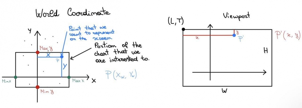
With the Window to Viewport Transformation, our goal is to transform the real-world coordinates (i.e. pair of x and y that indicate respectively the coordinate on the x-axis and on the y one) to the viewport ones (the screen coordinates).
As a first step, we have to identify the real-world window which we want to project in our viewport because we may be interested in specific portions of our real-world chart and this is useful to maintain its original shape. How can we do this? We can easily obtain this with a linear transform: in practice, it’s like we consider the real-world window and we stretch or shrink it to fit inside the viewport.
The coordinates of the viewport on the screen are completely different from the real-world window: in the first case, we are measuring pixels, in the second one we are measuring two variables that could have different units of measure. So we need to know how to transform each point in the real world (x_w, y_w) to a viewport point (x_d, y_d); first of all, remind that the origin of device points isn’t in the bottom-left corner, but in the top -left, therefore the y axis on the device is flipped respect to the cartesian system
What we want to find are 2 functions that given the real-world point give us its x and y to represent that point in the viewport:
To find those functions that can solve our problem, we need to keep track of the viewport size and also of the coordinates of its top-left corner that we indicate with (L, T); for what regards the real world, we will need: MinX, MinY, MaxX and MaxY.
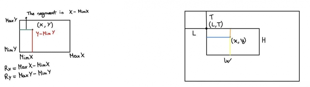
What is written below refers to this image above.
The green segment should correspond to the blue one: for instance, if the green segment is 1/3 of the Rx, we want also that the blue one will be 1/3 of W in order to maintain the proportion. So, (x – MinX)/Rx is the proportion factor which, if multiplied by W, will give us the blue segment; however, to obtain viewport x, we have to add to our blue segment L.
To conclude, viewport x will be given by the following:
The same can be done for Y, paying attention to the fact that the y-axis is flipped in the viewport with respect to the cartesian system.
The proportion of the red segment is: (y – MinY)/Ry, which multiplied by H, gives us the yellow segment.
What we are searching for, though, isn’t the yellow segment, but the orange one.
So, how could we obtain the orange segment? It’s just H – yellowSegment, i.e. H – H * (y – MinY)/Ry, and adding T we obtain the viewport y.
Here’s the formula to obtain the viewport y:
Useful coding for the conversion from a real point to the viewport one:
A measure of central tendency is a single value that attempts to describe a set of data by identifying the central position within that set of data. As such, measures of central tendency are sometimes called measures of central location. They are also classed as summary statistics. The mean (often called the average) is most likely the measure of central tendency that you are most familiar with, but there are others, such as the median and the mode.
The mean, median, and mode are all valid measures of central tendency, but under different conditions, some measures of central tendency become more appropriate to use than others. Below, we will look at the mean, mode, and median, and understand how to calculate them and under what conditions they are most appropriate to be used.
Mean (or Avarage)
The (arithmetic) mean, or average, of n observations x_bar is simply the sum of the observations divided by the number of observations; thus:
In this equation, xi represents the individual sample values and Σxi their sum.
Median
The median is defined as the middle point of the ordered data. It is estimated by first ordering the data from smallest to largest and then counting upwards for half the observations. The estimate of the median is either the observation at the center of the ordering in the case of an odd number of observations or the simple average of the middle two observations if the total number of observations is even.
There is an obvious disadvantage, the median uses the position of data points rather than their values. That way some valuable information is lost and we have to rely on other kinds of measures such as measures of dispersion to get more information about the data.
Mode
The third measure of location is the mode. This is the value that occurs most frequently, or, if the data are grouped, the grouping with the highest frequency. It may be useful for categorical data to describe the most frequent category. The expression ‘bimodal’ distribution is used to describe a distribution with two peaks in it. This can be caused by mixing populations.
Distance
The measures of central tendency are not adequate to describe data. Two data sets can have the same mean but they can be entirely different. Thus to describe data, one needs to know the extent of variability. This is given by the measures of dispersion. Is important because the smaller the dispersion, the more realistic the data. But to calculate the dispersion we have to define the distance.
In mathematic terms the distance is a numerical measurement of how far apart objects or points are; a distance function or metric is a generalization of the concept of physical distance; it is a way of describing what it means for elements of some space to be “close to”, or “far away from” each other.
In machine learning, a distance measure is an objective score that summarizes the relative difference between two objects in a problem domain. Most commonly, the two objects are rows of data that describe a subject (such as a person, car, or house), or an event (such as a purchase, a claim, or a diagnosis).
In Statistics, distance is a measure calculated between two records that are typically part of a larger dataset, where rows are records and columns are variables.
There are different kinds of distances:
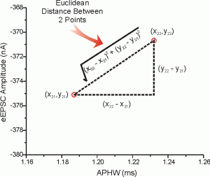
1. Euclidian Distance :
It is a distance measure that best can be explained as the length of a segment connecting two points. The formula is rather straightforward as the distance is calculated from the cartesian coordinates of the points using the Pythagorean theorem.
Euclidean distance works great when you have low-dimensional data and the magnitude of the vectors is important to be measured.
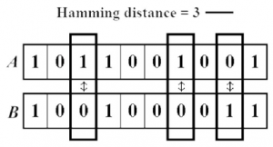
2. Hamming Distance:
Hamming distance is the number of values that are different between two vectors. It is typically used to compare two binary strings of equal length. It can also be used for strings to compare how similar they are to each other by calculating the number of characters that are different from each other:
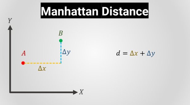
3. Manhattan Distance:
The Manhattan distance calculates the distance between real-valued vectors. Imagine vectors that describe objects on a uniform grid such as a chessboard. Manhattan distance then refers to the distance between two vectors if they could only move right angles. There is no diagonal movement involved in calculating the distance:
All these distances can be used in different subjects such as machine learning, data science, mathematics; but obviously, they will give different results because each of them has a different declaration of distance.
https://emanueleseminara.it/wp-content/uploads/2021/10/Statistics_researches_5_R.png705705zifrohttps://emanueleseminara.it/wp-content/uploads/2021/09/logo.pngzifro2021-10-22 12:10:152021-11-08 13:50:17Research about theory 5_R
5_R. Explain a possibly unified conceptual framework to obtain all most common measures of central tendency and of dispersion using the concept of distance (or “premetric”, or similarity in general). Discuss why it is useful to discuss these concepts introducing the notion of distance. Finally, point out the difference between the mathematical definition of “distance” and the properties of the “premetrics” useful in statistics, pointing out trhe most important distances, indexes and similarity measures used in statistics, data analysis and machine learning (such as for instance; Mahalanobis distance, Euclidean distance, Minkowski distance, Manhattan distance, Hamming distance, Cosine distance, Chebishev distance, Jaccard index, Haversine distance, Sørensen-Dice index, etc.).
6_A. (For this exercises use only 1 language chosen between C# or VB.NET, according to your preference)
Prepare separately the following charts: 1) Scatterplot, 2) Histogram/Column chart [in the histogram, within each class interval, draw also a vertical colored line where lies the true mean of the observations falling in that class] and 3) Contingency table, using the graphics object and its methods (Drawstring(), MeasureString(), DrawLine(), etc).
Use them to represent 2 numerical variables that you select from a CSV file. In particular, in the same picture box, you will make at least 2 separate charts: 1 dynamic rectangle will contain the contingency table, and 1 rectangle (chart) will contain the scatterplot, with the histograms/column charts and rug plots drawn respectively near the two axis (and oriented accordingly).
4_RA. Do a personal research about the real world window to viewport transformation, and note separately the formulas and code which can be useful for your present and future applications.
This video showing how application 1_A works (in both C # and vb-net).
The form is composed by:
a buttons;
a TextBox;
a pictureBox.
Pressing the “Show word cloud” button the .txt file specified in the textBox is loaded, the words with higher frequency in the text differentiated by size and color are printed in the pictureBox.
This video showing how application 1_A works (in both C # and vb-net).
The form is composed by:
a buttons;
two label;
two textBox;
a richTextBox.
Pressing the “Load CSV” key the .csv file specified in the textBox is loaded, its content is printed in the richTextBox and finally, the mean, the standard deviation and the distribution are displayed.
We may request cookies to be set on your device. We use cookies to let us know when you visit our websites, how you interact with us, to enrich your user experience, and to customize your relationship with our website.
Click on the different category headings to find out more. You can also change some of your preferences. Note that blocking some types of cookies may impact your experience on our websites and the services we are able to offer.
Essential Website Cookies
These cookies are strictly necessary to provide you with services available through our website and to use some of its features.
Because these cookies are strictly necessary to deliver the website, refuseing them will have impact how our site functions. You always can block or delete cookies by changing your browser settings and force blocking all cookies on this website. But this will always prompt you to accept/refuse cookies when revisiting our site.
We fully respect if you want to refuse cookies but to avoid asking you again and again kindly allow us to store a cookie for that. You are free to opt out any time or opt in for other cookies to get a better experience. If you refuse cookies we will remove all set cookies in our domain.
We provide you with a list of stored cookies on your computer in our domain so you can check what we stored. Due to security reasons we are not able to show or modify cookies from other domains. You can check these in your browser security settings.
Other external services
We also use different external services like Google Webfonts, Google Maps, and external Video providers. Since these providers may collect personal data like your IP address we allow you to block them here. Please be aware that this might heavily reduce the functionality and appearance of our site. Changes will take effect once you reload the page.
Google Webfont Settings:
Google Map Settings:
Google reCaptcha Settings:
Vimeo and Youtube video embeds:
Privacy Policy
You can read about our cookies and privacy settings in detail on our Privacy Policy Page.

![\[ P(A|B)=\frac{P(B|A)P(A)}{P(B)} \]](https://emanueleseminara.it/wp-content/ql-cache/quicklatex.com-f1a041584951e962ba9a4f3bc776da6e_l3.png "Rendered by QuickLaTeX.com")

 is a conditional probability: the probability of event
  occurring given that
  is true. It is also called the posterior probability of
  is also a conditional probability: the probability of event
  .
. and
and  are the probabilities of observing


![\[ \begin{cases} x= f_x(x_w)\\ y=f_y(y_w) \\ \end{cases} \]](https://emanueleseminara.it/wp-content/ql-cache/quicklatex.com-2d81facabf1bd6790d766ddd9de4f409_l3.png "Rendered by QuickLaTeX.com")
![\[ x=L+\frac{x-x_{min}}{R_x}\cdot w \]](https://emanueleseminara.it/wp-content/ql-cache/quicklatex.com-7244a381fedf08d95591af1b229f78a3_l3.png "Rendered by QuickLaTeX.com")
![\[ y=T+H-\frac{y-y_{min}}{R_y}\cdot h \]](https://emanueleseminara.it/wp-content/ql-cache/quicklatex.com-7460564b211a3124bdcf7845e716bb60_l3.png "Rendered by QuickLaTeX.com")
![\[\bar{x}=\sum \frac{x_i}{n}\]](https://emanueleseminara.it/wp-content/ql-cache/quicklatex.com-950b7b3efc2307fe4e3744ee34bd1bda_l3.png "Rendered by QuickLaTeX.com")
![\[D(x, y)=\sqrt{\sum_{i=1}^n (x_i-y_i)^2}\]](https://emanueleseminara.it/wp-content/ql-cache/quicklatex.com-67b4d5709eb12fed6e00f6e67f6c196e_l3.png "Rendered by QuickLaTeX.com")