Researches about theory

12_R.What is the “Brownian motion” and what is a Wiener process. History, importance, definition and applications (Bachelier, Wiener, Einstein, …).


13_R. An “analog” of the CLT for stochastic process: the standard Wiener process as “scaling limit” of a random walk and the functional CLT (Donsker theorem) or invariance principle. Explain the intuitive meaning of this result and how you have already illustrated the result in your homework.


Applications

12_A. Discover one of the most important stochastic process by yourself!

Consider the general scheme we have used so far to simulate stochastic processes (such as the relative frequency of success in a sequence of trials, the sample mean, the random walk, the Poisson point process, etc.) and now add this new process to our simulator.

Starting from value 0 at time 0, for each of m paths, at each new time compute P(t) = P(t-1) + Random step(t), for t = 1, …, n,
where the Random step(t) is now:

σ * sqrt(1/n) * Z(t),

where  Z(t) is a N(0,1) random variable (the “diffusion” σ is a user parameter, to scale the process dispersion).
At time n (last time) and one (or more) other chosen inner time 1.


13_A. Create the a distribution representation (histogram, or CDF …) to represent the following:

– Realizations taken from a Normal(0,1)

– Realizations of the mean, obtained by averaging several times (say m times, m large) n of the above realizations
– Realizations of the variance, obtained by averaging several times (say m times, m large) n of the above realizations

– Realizations taken from exp(N(0,1)))

– Realizations taken from N(0,1) squared

– Realizations taken from a (squared N(0,1)) divided by another (squared N(0,1)).


Researches about applications

9_RA Try to find on the web what are the names of the random variables that you just simulated in the applications, and see if the means and variances that you obtain in the simulation are compatible with the “theory”. If not fix the possible bugs.


Researches about theory

10_R. Distributions of the order statistics: look on the web for the most simple (but still rigorous) and clear derivations of the distributions, explaining in your own words the methods used.


11_R. Do a research about the general correlation coefficient for ranks and the most common indices that can be derived by it. Do one example of computation of these correlation coefficients for ranks.


Applications

10_A. Given a random variable, extract m samples of size n and plot the empirical distribution of its mean (histogram), the first and the last order statistics. Comment on what you see.


11_A. Discover a new important stochastic process by yourself! Consider the general scheme we have used so far to simulate some stochastic processes (such as the relative frequency of success in a sequence of trials, the sample mean and the random walk) and now add this new process to our process simulator.

Same scheme as previous program (random walk), except changing the way to compute the values of the paths at each time. Starting from value 0 at time 0, for each of m paths, at each new time compute N(i) = N(i-1) + Random step(i), for i = 1, …, n, where Random step(i) is now a Bernoulli random variable with success probability equal to λ * (1/n)  (where λ is a user parameter, eg. 50, 100, …).

At time n (last time) and one (or more) other chosen inner time 1

Represent also the distributions of the following quantities (and any other quantity that you think of interest):
– Distance (time elapsed) of individual jumps from the origin
– Distance (time elapsed) between consecutive jumps (the so-called “holding times”)


Researches about applications

8_RA. Find out on the web what you have just generated in the previous application. Can you find out about all the well known distributions that “naturally arise” in this process ?


Researches about theory

9_R.  History and derivation of the normal distribution. Touch, at least, the following three i mportant perspectives, putting them into an historical context to understand how  the idea developed:

1) as approximation of binomial (De Moivre)
2) as error curve (Gauss)
3) as limit of sum of independent r.v.’s (Laplace)


Applications

9_A_1. Create a simulation with graphics to convince yourself of the pointwise convergence of the empirical CDF to the theoretical distribution (Glivenko-Cantelli theorem). Use a simple random variable of your chooice for such a demonstration.

PlotEmpiricalCdfAndCompareWithSamplingDistributionExample_01(source: https://it.mathworks.com/help/stats/cdfplot.html )


9_A_2.  Generate sample paths of jump processes which at each time considered t = 1, …, n perform jumps computed as:

–   σ sqrt(1/n) R(t)
where R(t)  is a [-1,1] Rademacher random variable (https://en.wikipedia.org/wiki/Rademacher_distribution).

–  σ sqrt(1/n) * Z(t), where  Z(t) is a N(0,1) random variable (https://en.wikipedia.org/wiki/Normal_distribution)

and see what happens as n (simulation parameter) becomes larger.

[As before, at time n (last time) and one other chosen inner time 1 (source: https://www.datatime.eu/public/StatApp2020/ )


Researches about applications

7_RA Do a research about the random walk process and its properties. Compare your finding with your applications drawing your personal conclusions. Explain based on your exercise the beaviour of the distribution of the stochastic process (check out “Donsker’s invariance principle”). What are, in particular, its mean and variance at time n ?


Researches about theory

8_R.

Do a research about the following topics:

– The law of large numbers LLN, the various definitions of convergence

– The convergence of the Binomial to the normal and Poisson distributions

– The central limit theorem [in anticipation of a topic we will study later]


Applications

8_A. Exercise (also partially described in video 04)

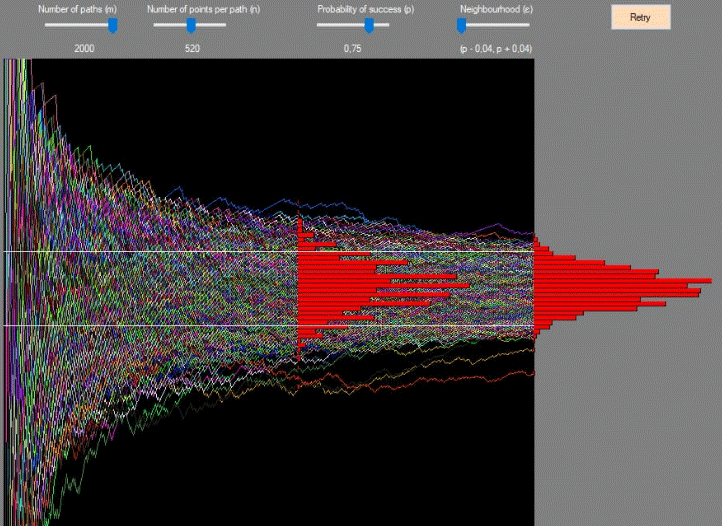
Generate and represent m “sample paths” of n point each (m, n are program parameters), where each point represents a pair of:

time index t, and relative frequency of success f(t),

where f(t) is the sum of t Bernoulli random variables with distribution B(x, p) = p^x(1-p)^(1-x) observed at the various times up to t: j=1, …, t..

At time n (last time) and one other chosen inner time 1f(t) with the absolute frequency n(t) or by normalized relative frequency: f(t) / sqrt(p(1-p)/n).

Comment briefly on the result.

Empirical Freqency Sample Paths    (courtesy: homework screenshot by Lorenzo Zara, year 2020)

(The general scheme of this exercise, will also be “reused” in next homeworks where we will consider other more interesting stochastic processes.)


Researches about applications

6_RA. Do a web research about the various methods proposed to compute the running median (one pass, online algorithms).
Store (cite all sources and attributions) the algorithm(s) that you think is(are) a good candidate, explaining briefly how it works and possibly try a quick demo.


Researches about theory

6_R. Think and explain in your own words what is the role that probability plays in Statistics and the relation between the observed distribution and frequencies their “theoretical” counterparts. Do some practical examples where you explain how the concepts of an abstract probability space relate to more “concrete” and “real-world” objects when doing statistics.


7_R. Explain the Bayes Theorem and its key role in statistical induction. Describe the different paradigs that can be found within statistical inference (such as”bayesian”, “frequentist” [Fisher, Neyman]).


Applications

7_A. Given 2 variables from a csv compute and represent the statistical regression lines (X to Y and viceversa) and the scatterplot.
Optionally, represent also the histograms on the “sides” of the chart (one could be draw vertically and the other one horizontally, in the position that you prefer).
[Remember that all our charts must alway be done within “dynamic viewports” (movable/resizable rectangles). No third party libraries, to ensure ownership of creative process. May choose the language you prefer.].


Researches about applications

5_RA. Do a web research about the various methods to generate, from a Uniform([0,1)), all the most important random variables (discrete and continuous). Collect all source code you think might be useful code of such algorithms (keep credits and attributions wherever applicable), as they will be useful for our next simulations.


Researches about theory

5_R. Explain a possibly unified conceptual framework to obtain all most common measures of central tendency and of dispersion using the concept of distance (or “premetric”, or similarity in general). Discuss why it is useful to discuss these concepts introducing the notion of distance. Finally, point out the difference between the mathematical definition of “distance” and the properties of the “premetrics” useful in statistics, pointing out trhe most important distances, indexes and similarity measures used in statistics, data analysis and machine learning (such as for instance; Mahalanobis distance, Euclidean distance, Minkowski distance, Manhattan distance, Hamming distance, Cosine distance, Chebishev distance, Jaccard index, Haversine distance, Sørensen-Dice index, etc.).


Applications

6_A. (For this exercises use only 1 language chosen between C# or VB.NET, according to your preference)

Prepare separately the following charts: 1) Scatterplot, 2) Histogram/Column chart [in the histogram, within each class interval, draw also a vertical colored line where lies the true mean of the observations falling in that class] and 3) Contingency table, using the graphics object and its methods (Drawstring(), MeasureString(), DrawLine(), etc).
Use them to represent 2 numerical variables that you select from a CSV file. In particular, in the same picture box, you will make at least 2 separate charts: 1 dynamic rectangle will contain the contingency table, and 1 rectangle (chart) will contain the scatterplot, with the histograms/column charts and rug plots drawn respectively near the two axis (and oriented accordingly).


Researches about applications

4_RA. Do a personal research about the real world window to viewport transformation, and note separately the formulas and code which can be useful for your present and future applications.


Optional applications

Translate the last exercises 6_A to web browser applications, in plain javascript (no “third party libraries”,  check also
https://www.datatime.eu/public/cybersecurity/JSTutorial/ for some progressive examples)


Researches about theory

4_R. Explain what are marginal, joint and conditional distributions and how we can explain the Bayes theorem using relative frequencies. Explain the concept of statistical independence and why, in case of independence, the relative joint frequencies are equal to the products of the corresponding marginal frequencies.


Applications

4_A. Create a program – in both languages C# and VB.NET (and optionally in js) – to read data from a CSV file, and store it into a suitable collection of suitably designed objects, for further processing. Compute mean and standard deviation and frequency distribution for at least one of the variable, and for one pair of variables.


5_A. Compute – in both languages C# and VB.NET (and optionally in js) – a frequency distribution of the meaningful words from any text file and create a personal graphical representation of the corresponding “word cloud” (in case, can use animation if you wish), keeping into account the frequencies of the words.


Researches about applications

2_RA. Do a review about charts useful for statistics and data presentation (example of some: StatCharts.txt ). What is the chart type that impressed you most and why ?


3_RA. Do a comprehensive research about the GRAPHICS object and all its members (to get ready to create any statistical chart.)


Researches about theory

2_R. Describe the most common configuration of data repositories in the real world and corporate environment. Concepts such as Operational or Transactional systems (OLTP), Data Warehouse DW, Data Marts, Analytical and statistical systems (OLAP), etc. Try to draw a conceptual picture of how all these components may work together and how the flow of data and information is processed to extract useful knowledge from raw data.


3_R. Show how we can obtain an online algo for the arithmetic mean and explain the various possible reasons why it is preferable to the “naive” algo based on the definition.


Applications

2_A. Create – in both languages C# and VB.NET – a demonstrative program which computes the online arithmetic mean (if it’s a numeric variable) and your own algo to compute the distribution for a discrete variable and for a continuous variable (can use values simulated with RANDOM object).


3_A. Create an object providing a rectangular area which can be moved and resized using the mouse. This area will hold our future charts and graphics.


Researches about applications

1_RA. Understand how the floating point representation works and describe systematically (possibly using categories) all the possible problems that can happen. Try to classify the various issues and limitations (representation, comparison, rounding, propagation, approximation, loss of significance, cancellation, etc.) and provide simple examples for each of the categories you have identified.


Researches about theory

1_R. Give your best description of the many reaching out of statistics, in its various form, as a branch of math (Probability theory, etc.), as a set of methodologies used in many other disciplines, as an essential tool to deal with any sort of data, make reports and provide governance tools. Discuss whether it can be considered a “science” and what is the “scientific method” (what is a “theory” and what is a “hypothesis”). What is the role of Statistics in Math and Science?


Applications

1_A. Create – in both languages C# and VB.NET – a program which does the following simple tasks to get acquainted with the tool:

– when a button is pressed some text appears in a richtexbox on the startup form
– when another button is pressed animate one or more balls (possibly of different colors and sizes) within a rectangle