Statistics – Emanuele Seminara

Researches, Statistics

Research about applications 9_RA

In application 13_A we simulated the following random variables

November 28, 2021/0 Comments/by zifro

Applications, Statistics

Application 13_A

Download C#

November 28, 2021/0 Comments/by zifro

Applications, Statistics

Application 12_A

Download C#

November 28, 2021/0 Comments/by zifro

Researches, Statistics

A quick recap about CLT

In probability theory, the central limit theorem (CLT) states that the distribution of a sample variable approximates a normal distribution (i.e., a “bell curve”) as the sample size becomes larger, assuming that all samples are identical in size, and regardless of the population’s actual distribution shape.

Put another way, CLT is a statistical premise that, given a sufficiently large sample size from a population with a finite level of variance, the mean of all sampled variables from the same population will be approximately equal to the mean of the whole population. Furthermore, these samples approximate a normal distribution, with their variances being approximately equal to the variance of the population as the sample size gets larger, according to the law of large numbers.

Introduction to Wiener Process (also called Brownian Motion)

The concept of a Brownian motion was discovered when Einstein observed particles oscillating in liquid. Since fluid dynamics are so chaotic and rapid at the molecular level, this process can be modelled best by assuming the particles move randomly and independently of their past motion. We can also think of Brownian motion as the limit of a random walk as its time and space increments shrink to 0. In addition to its physical importance,
Brownian motion is a central concept in stochastic calculus.

Definition of Wiener Process

A standard (one-dimensional) Wiener process (also called Brownian motion) is a stochastic process $\left \{ W_t \right \}_{t\geq 0}$ indexed by nonnegative real numbers t with the following properties:

$W_0$ = 0.
With probability 1, the function t → Wt is continuous in t.
The process $\left \{ W_t \right \}_{t\geq 0}$ has stationary, independent increments.
The increment $W_{t+s} − W_s$ has the $NORMAL(0, t)$ distribution.

Wiener Process as a scaling limit of Random Walks

One of the many reasons that Brownian motion is important in probability theory is that it is, in a certain sense, a limit of rescaled simple random walks. Let $ξ_1, ξ_2, …$ be a sequence of independent, identically distributed random variables with mean 0 and variance 1. For each $n\geq 1$ define a continuous-time stochastic process $\left \{ W_{n(t)} \right \}_{t\geq 0}$ by:

This is a random step function with jumps of size $\pm 1\sqrt{n}$ at times $V$ , where $k\in \mathbb{Z}^+$ . Since the random variables $ξ_j$ are independent, the increments of $W_{n(t)}$ are independent. Moreover, for large n the distribution of $W_n(t + s) − W_n(s)$ is close to the $NORMAL(0, t)$ distribution, by the Central Limit theorem. Thus, it requires only a small leap of faith to believe that, as $n\rightarrow \infty$ , the distribution of the random function $W_n(t)$ approaches (in a sense made precise below) that of a standard Brownian motion.
Why is this important? First, it explains, at least in part, why the Wiener process arises so commonly in nature. Many stochastic processes behave, at least for long stretches of time, like random walks with small but frequent jumps. The argument above suggests that such processes will look, at least approximately, and on the appropriate time scale, like Brownian motion.
Second, it suggests that many important “statistics” of the random walk will have limiting distributions and that the limiting distributions will be the distributions of the corresponding statistics of Brownian motion. The simplest instance of this principle is the central limit theorem: the distribution of $W_n(1)$ is, for large n close to that of $W(1)$ (the gaussian distribution with mean 0 and variance 1). Other important instances do not follow so easily from the central limit theorem. For example, the distribution of:

converges, as $n\rightarrow \infty$ , to that of:

Donsker’s Theorem

In probability theory, Donsker’s theorem (also known as Donsker’s invariance principle, or the functional central limit theorem), named after Monroe D. Donsker, is a functional extension of the central limit theorem.

Let $X_1, X_2, X_3, \ldots$ be a sequence of independent and identically distributed (i.i.d.) random variables with mean 0 and variance 1.

Let $S_n:=\sum_{i=1}^n X_i$ .

The stochastic process $S:=(S_n)_{n\in\N}$ is known as a random walk. Define the diffusively rescaled random walk (partial-sum process) by

W^{(n)}(t) := \frac{S_{\lfloor nt\rfloor}}{\sqrt{n}}, \qquad t\in [0,1].

The central limit theorem asserts that $W^{(n)}(1)$ converges in distribution to a standard Gaussian random variable $W(1)$ as $n\to \infty$ . Donsker’s invariance principle extends this convergence to the whole function $W^{(n)}:=(W^{(n)}(t))_{t\in [0,1]}$ . More precisely, in its modern form, Donsker’s invariance principle states that: As random variables taking values in the Skorokhod space* $\mathcal{D}[0,1]$ , the random function $W^{(n)}$ converges in distribution to a standard Brownian motion $W:=(W(t))_{t\in [0,1]}$ as $n\to \infty$

*The set of all càdlàg functions from E to M is often denoted by D(E; M) (or simply D) and is called Skorokhod space after the Ukrainian mathematician Anatoliy Skorokhod.

References

Càdlàg – Wikipedia

Donsker’s theorem – Wikipedia

BrownianMotionCurrent.pdf (uchicago.edu)

Dahl.pdf (uchicago.edu)

Central Limit Theorem (CLT) Definition (investopedia.com)

November 23, 2021/0 Comments/by zifro

HomeWork, Statistics

Homework 9

Researches about theory

12_R.What is the “Brownian motion” and what is a Wiener process. History, importance, definition and applications (Bachelier, Wiener, Einstein, …).

Go to research

13_R. An “analog” of the CLT for stochastic process: the standard Wiener process as “scaling limit” of a random walk and the functional CLT (Donsker theorem) or invariance principle. Explain the intuitive meaning of this result and how you have already illustrated the result in your homework.

Go to research

Applications

12_A. Discover one of the most important stochastic process by yourself!

Consider the general scheme we have used so far to simulate stochastic processes (such as the relative frequency of success in a sequence of trials, the sample mean, the random walk, the Poisson point process, etc.) and now add this new process to our simulator.

Starting from value 0 at time 0, for each of m paths, at each new time compute P(t) = P(t-1) + Random step(t), for t = 1, …, n,
where the Random step(t) is now:

σ * sqrt(1/n) * Z(t),

where Z(t) is a N(0,1) random variable (the “diffusion” σ is a user parameter, to scale the process dispersion).
At time n (last time) and one (or more) other chosen inner time 1.

Go to applicaton

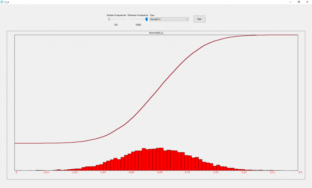
13_A. Create the a distribution representation (histogram, or CDF …) to represent the following:

– Realizations taken from a Normal(0,1)

– Realizations of the mean, obtained by averaging several times (say m times, m large) n of the above realizations
– Realizations of the variance, obtained by averaging several times (say m times, m large) n of the above realizations

– Realizations taken from exp(N(0,1)))

– Realizations taken from N(0,1) squared

– Realizations taken from a (squared N(0,1)) divided by another (squared N(0,1)).

Go to applicaton

Researches about applications

9_RA Try to find on the web what are the names of the random variables that you just simulated in the applications, and see if the means and variances that you obtain in the simulation are compatible with the “theory”. If not fix the possible bugs.

Go to research

November 23, 2021/0 Comments/by zifro

Researches, Statistics

Research about theory 12_R

The concept of a Brownian motion was discovered when Einstein observed particles oscillating in liquid. Since fluid dynamics are so chaotic and rapid at the molecular level, this process can be modeled best by assuming the particles move randomly and independently of their past motion. We can also think of Brownian motion as the limit of a random walk as its time and space increments shrink to 0. In addition to its physical importance, Brownian motion is a central concept in stochastic calculus which can be used in finance and economics to model stock prices and interest rates.

What is Brownian motion and why are we interested?

Much of probability theory is devoted to describing the macroscopic picture emerging in random systems defined by a host of microscopic random effects. Brownian motion is the macroscopic picture emerging from a particle moving randomly in d-dimensional space without making very big jumps. On the microscopic level, at any time step, the particle receives a random displacement, caused for example by other particles hitting it or by an external force, so that, if its position at time zero is $S_0$ , its position at time n is given as $S_n=S_0+\sum ^n _{i=1}X_i$ , where the displacements $X_1, X_2, X_3, ...$ are assumed to be independent, identically distributed random variables with values in $\mathbb{R}^d$ . The process $\left \{ S_n:n\geq 0 \right \}$ is a random walk, the displacements represent the microscopic inputs. It turns out that not all the features of the microscopic inputs contribute to the macroscopic picture. Indeed, if they exist, only the mean and covariance of the displacements are shaping the picture. In other words, all random walks whose displacements have the same mean and covariance matrix give rise to the same macroscopic process, and even the assumption that the displacements have to be independent and identically distributed can be substantially relaxed. This effect is called universality, and the macroscopic process is often called a universal object. It is a common approach in probability to study various phenomena through the associated universal objects.

If the jumps of a random walk are sufficiently tame to become negligible in the macroscopic picture, in particular if it has finite mean and variance, any continuous time stochastic process $\left \{ B(t):t\geq 0 \right \}$ describing the macroscopic features of this random walk should have the following properties:

for all times $0\leq t_1\leq t_2\leq ...\leq t_n$ the random variables $B(t_n)-B(t_{n-1}), B(t_{n-1})-B(t_{n-2}), ..., B(t_2)-B(t_1)$ are independent; we say that the process has independent increments,
the distribution of the increment $B(t+h)-B(t)$ does not depend on $t$ ; we say that the process has stationary increments,
the process $\left \{ B(t):t\geq 0 \right \}$ has almost surely continuous paths.
for every $t\geq 0$ and $h\geq 0$ the increment $B(t+h)-B(t)$ is multivariate normally distributed with mean $h\mu$ and covariance matrix $h\Sigma \Sigma ^T$ .

Hence any process with the features (1)-(3) above is characterised by just three parameters,

the initial distribution, i.e. the law of $B(0)$ ,
the drift vestor $\mu$ ,
the diffusion matrix $\Sigma$ .

If the drift vector is zero, and the diffusion matrix is the identity we say the process is a Brownian motion. If $B(0)=0$ , i.e. the motion is started at the origin, we use the term standard Brownian motion.

Suppose we have a standard Brownian motion $\left \{ B(t):t\geq 0 \right \}$ . If $X$ is a random variable with values in $\mathbb{R}^d$ and $\Sigma$ a $d\times d$ matrix, then it is easy to check that $\left \{ \tilde{B}(t):t\geq 0 \right \}$ given by

$\tilde{B}(t)=X+\mu t+\Sigma B(t)$ , for $t\geq 0$ ,

is a process with the properties (1)-(4) with initial distribution $X$ , drift vestor $\mu$ and diffusion matrix $\Sigma$ . Hence the macroscopic picture emerging from a random walk with finite variance can be fully described by a standard Brownian motion.

References

lecnotes_moerters.pdf (math-berlin.de)

Dahl.pdf (uchicago.edu)

November 23, 2021/0 Comments/by zifro

Researches, Statistics

Research about applications 8_RA

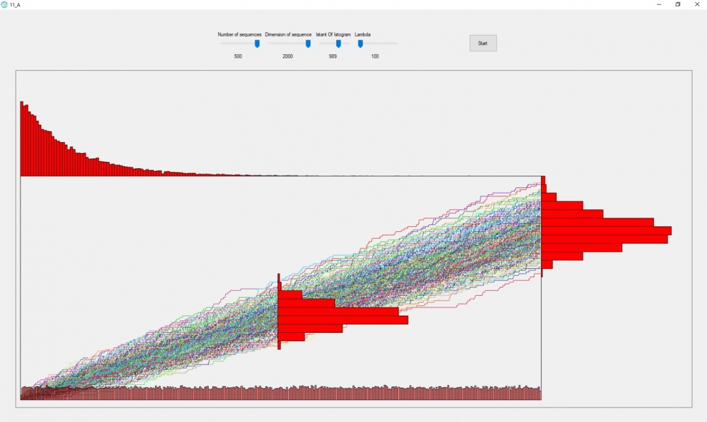
The previous graph is taken from application 11_A, as we can see the following distributions are present:

Poisson distribution
Uniform distribution
Exponential Distribution
Poisson process

A Poisson process is a model for a series of discrete events where the mean time between events is known, but the exact timing of the events is random. The arrival of an event is independent of the previous event. The important point is that we know the mean time between events but they are randomly spaced (stochastic). We could have consecutive failures, but we could also spend years between failures due to the randomness of the process.

A Poisson process satisfies the following criteria (in reality many phenomena modeled as Poisson processes do not exactly satisfy them):

Events are independent of each other. The occurrence of one event does not affect the likelihood of another event occurring.
The average rate (events per time period) is constant.
Two events cannot occur at the same time. It means that we can think of any sub-interval of a Poisson process as a Bernoulli test, i.e. a success or a failure.

Poisson distribution

The Poisson process is the model we use to describe randomly occurring events. Using the Poisson Distribution we could find the probability of a number of events over a period of time or find the probability of waiting some time until the next event.

The probability function of the Poisson distribution gives the probability of observing k events over a period of time given the length of the period and the time-averaged events:

This is a little convoluted, and events/time * time period is usually simplified into a single parameter, λ, lambda, the rate parameter. With this substitution, the Poisson Distribution probability function now has one parameter:

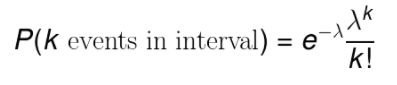
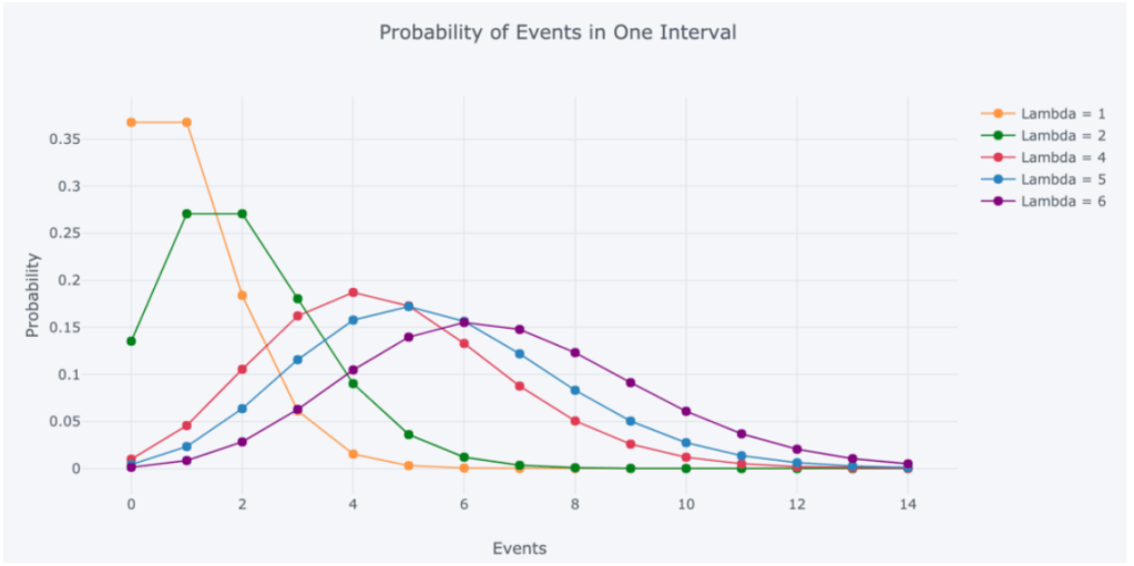
Lambda can be thought of as the expected number of events in the interval.

When we change the parameter λ we change the probability of seeing different numbers of events in an interval. The graph below is the probability mass function of the Poisson distribution which shows the probability of a number of events occurring in an interval with different velocity parameters.

References

The Poisson Distribution and Poisson Process Explained | by Will Koehrsen | Towards Data Science

November 21, 2021/0 Comments/by zifro

Applications, Statistics

Application 11_A

Download C#

November 21, 2021/0 Comments/by zifro

Researches, Statistics

Research about theory 10_R

Order statistics are a very useful concept in statistical sciences. They have a wide range of applications including modelling auctions, car races, and insurance policies, optimizing production processes, estimating parameters of distributions, and so forth.
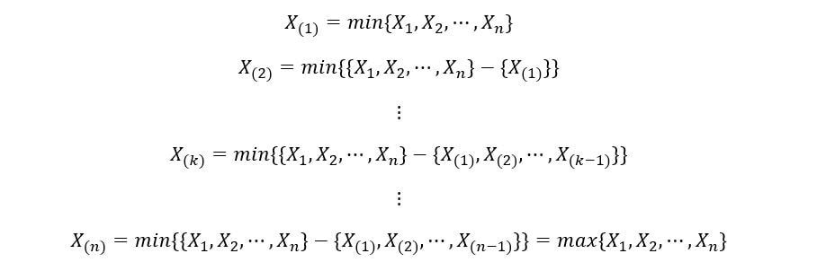
Suppose we have a set of random variables X₁, X₂, …, X_n, which are independent and identically distributed (i.i.d). By independence, we mean that the value taken by a random variable is not influenced by the values taken by other random variables. By identical distribution, we mean that the probability density function (PDF) (or equivalently, the Cumulative distribution function, CDF) for the random variables is the same. The k^th order statistic for this set of random variables is defined as the k^th smallest value of the sample.

To better understand this concept, we’ll take 5 random variables X₁, X₂, X₃, X₄, X₅. We’ll observe a random realization/outcome from the distribution of each of these random variables. Suppose we get the following values:

The k^th order statistic for this experiment is the k^th smallest value from the set {4, 2, 7, 11, 5}. So, the 1^st order statistic is 2 (smallest value), the 2^nd order statistic is 4 (next smallest), and so on. The 5^th order statistic is the fifth smallest value (the largest value), which is 11. We repeat this process many times i.e., we draw samples from the distribution of each of these i.i.d random variables, & find the k^th smallest value for each set of observations. The probability distribution of these values gives the distribution of the k^th order statistics.

In general, if we arrange random variables X₁, X₂, …, X_n in ascending order, then the k^th order statistic is shown as:

The general notation of the k^th order statistic is X_(k). Note X_(k) is different from X_k. X_k is the k^th random variable from our set, whereas X_(k) is the k^th order statistic from our set. X_(k) takes the value of X_k if X_k is the k^th random variable when the realizations are arranged in ascending order.

The 1^st order statistic X₍₁₎ is the set of the minimum values from the realization of the set of ‘n’ random variables. The n^th order statistic X_(n) is the set of the maximum values (nth minimum values) from the realization of the set of ‘n’ random variables. They can be expressed as:

Distribution of Order Statistics

We’ll now try to find out the distribution of order statistics. We’ll first describe the distribution of the n^th order statistic, then the 1^st order statistic & finally the k^th order statistic in general.

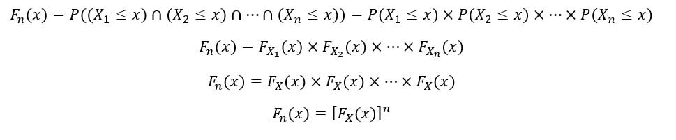
A) Distribution of the n^th Order Statistic:

Let the probability density function (PDF) & cumulative distribution function (CDF) our random variables be f_x(x), and F_x(x) respectively. By definition of CDF,

Since our random variables are identically distributed, they have the same PDF f_x(x) & CDF F_x(x). We’ll now calculate the CDF of n^th order statistic (F_n(x)) as follows:

The random variables X₁, X₂, …, X_n are also independent. Therefore, by property of independence,

The PDF of the n^th order statistic (f_n(x)) is calculated as follows:

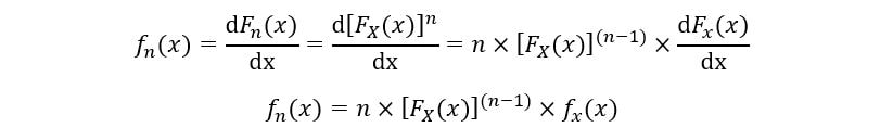
Thus, the expression for the PDF & CDF of n^th order statistic has been obtained.

B) Distribution of the 1^st Order Statistic:

The CDF of a random variable can also be calculated as the one minus the probability that the random variable X takes a value more than or equal to x. Mathematically,

We’ll determine the CDF of 1^st order statistic (F₁(x)) as follows:

We’ll determine the CDF of 1st order statistic (F1(x)) as follows

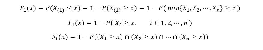
Once again, using the property of independence of random variables,

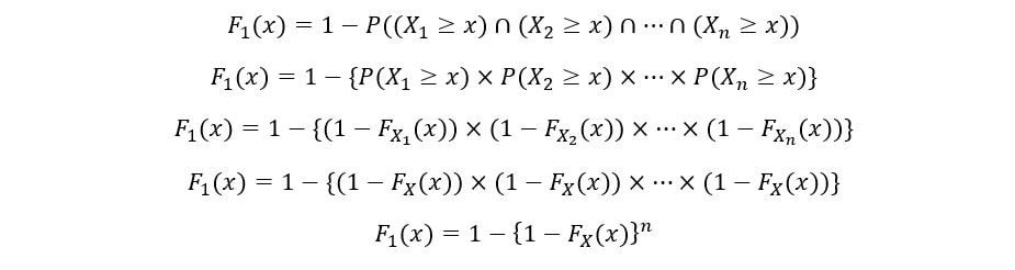
The PDF of the 1^st order statistic (f₁(x)) is calculated as follows:

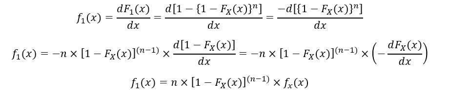
Thus, the expression for PDF & CDF of 1^st order statistic has been obtained.

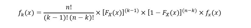
C) Distribution of the k^th Order Statistic:

For k^th order statistic, in general, the following equation describes its CDF (F_k(x)):

The PDF of k^th order statistic (f_k(x)) is expressed as:

To avoid confusion, we’ll use geometric proof to understand the equation. As discussed before, the set of random variables have the same PDF (f_X(x)). The following graph shows a sample PDF with the k^th order statistic obtained from random sampling:

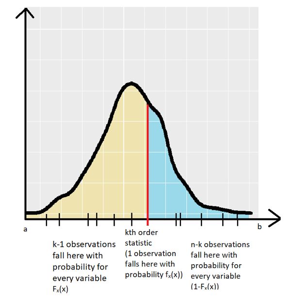
So, the PDF of the random variables f_X(x) is defined between the interval [a,b]. The kth order statistic for a random sample is shown by the red line. The other variable realizations (for the random sample) are shown by the small black lines on the x-axis.

There are exactly (k – 1) random variable observations that fall in the yellow region of the graph (the region between a & k^th order statistic). The probability that a particular observation falls in this region is given by the CDF of the random variables (F_X(x)). But we are aware that (k – 1) observations did fall in the region, which gives us the term (by independence) (F_X(x))^{(k – 1)}.

There are exactly (n – k) random variable observations that fall in the blue region of the graph (the region between k^th order statistic & b). The probability that a particular observation falls in this region is given by the 1 – CDF of the random variables (1– F_X(x)). But we are aware that (n – k) observations did fall in the region, which gives us the term (by independence) (1–F_X(x))^{(n – k)}.

Finally, exactly 1 observation falls exactly at the kth order statistic with probability f_X(x). Thus, the product of the 3 terms gives us an idea of the geometric meaning of the equation for PDF of the kth order statistic. But where does the factorial term come from? The above scenario just showed one of the many orderings. There can be many such combinations. The total number of such combinations is shown as follows:

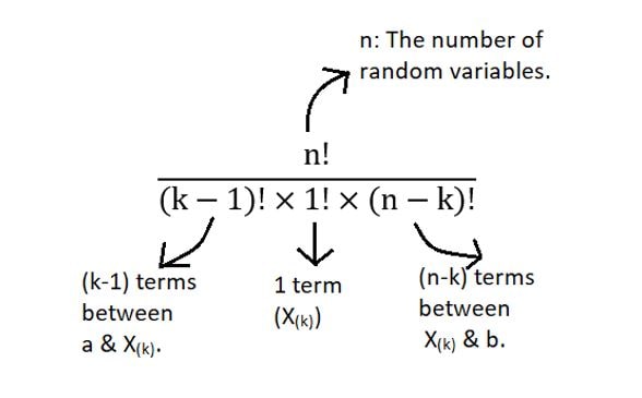
Thus, the product of all of these terms gives us the general distribution of the k^th order statistic.

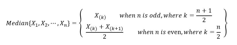
Useful Functions of Order Statistics

Order statistics give rise to various useful functions. Among them, the notable ones include sample range and sample median.

1) Sample range: It is defined as the difference between the largest and smallest value. It is expressed as follows:

2) Sample median: The sample median divides the random sample (realizations from the set of random variables) into two halves, one that contains samples with lower values, and the other that contains the samples with higher values. It’s like the middle/central order statistic. It is mathematically defined as:

Joint PDF of Order Statistics

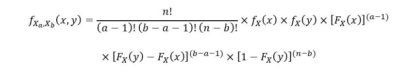
A joint probability density function can help us better understand the relationship between two random variables (two order statistics in our case). The joint PDF for any 2 order statistics X_(a) & X_(b), such that 1 ≤ a ≤ b ≤ n is given by the following equation:

References

Order Statistics | What is Order Statistics | Introduction to Order Statistics (analyticsvidhya.com)

November 21, 2021/0 Comments/by zifro

HomeWork, Statistics